Bayesian Learning in a Linear Basis Function Model

In this notebook we ilustrate the bayesian learning in a linear basis function model, as well as the sequential update of a posterior distribution.

Taken from Christopher Bishop’s Pattern Recognition and Machine Learning book (p.155)

import numpy as np
import matplotlib.pyplot as plt
from scipy.stats import multivariate_normal, norm
from numpy.random import seed, uniform, randn
from numpy.linalg import inv

%config InlineBackend.figure_format = "retina"

We consider an input \(x\), a target variable \(t\) and a linear model of the form \[ y(x, {\bf w}) = w_0 + w_1x \]

def f(x, a): return a[0] + a[1] * x

seed(314)
a = np.array([-0.3, 0.5])
N = 30
sigma = 0.2
X = uniform(-1, 1, (N, 1))
T = f(X, a) + randn(N, 1) * sigma

# plot_sample_w(0, )

plt.scatter(X, T, c="crimson")
plt.grid(alpha=0.5)
plt.plot(X, f(X,a))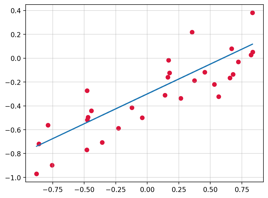

Our goal is to recover the values \(w_0\) and \(w_1\) from the data.

Recall: \[ p({\textbf w}|t) \propto p(t| {\textbf w}, \beta) p(\bf{w}) \]

beta = (1 / sigma) ** 2 # precision
alpha = 2.0

• \(t \sim \mathcal{N}\left({\bf w}^Tx, \beta^{-1}\right)\) (The assigned probability for target variables)

The posterior distribution of \(\bf w\) after \(N\) observations is given by

\[ \begin{align} m_N &= S_N(S_0^{-1}m_0 + \beta\Phi^T{\bf t}) \\ S_N^{-1} &= S_0^{-1} + \beta\Phi^T\Phi \end{align} \]

With * \(\Phi\in\mathbb{R}^{N\times M}\) * \({\bf t}\in\mathbb{R}^N\)

If no data has been yet seen, we consider \[ w \sim \mathcal{N}\left(0, \alpha^{-1}\text{I}\right) \] Which results in a posterior distribution of the form

\[ \begin{align} m_N &= \beta S_N\Phi^T{\bf t} \\ S_N^{-1} &= \alpha \text{I} + \beta\Phi^T\Phi \end{align} \]

def posterior_w(phi, t, S0, m0):
    """
    Compute the posterior distribution of 
    a Gaussian with known precision and conjugate
    prior a gaussian
    
    Parameters
    ----------
    phi: np.array(N, M)
    t: np.array(N, 1)
    S0: np.array(M, M)
        The prior covariance matrix
    m0: np.array(M, 1)
        The prior mean vector
    """
    SN = inv(inv(S0) + beta * Phi.T @ Phi)
    mN = SN @ (inv(S0) @ m0 + beta * Phi.T @ t)
    return SN, mN

def sample_vals(X, T, ix):
    """
    
    Returns
    -------
    Phi: The linear model transormation
    t: the target datapoint
    """
    x_in = X[ix]
    Phi = np.c_[np.ones_like(x_in), x_in] #  concatenate arrays along the second axis
    t = T[[ix]]
    return Phi, t

def plot_prior(m, S, liminf=-1, limsup=1, step=0.05, ax=plt, **kwargs):
    grid = np.mgrid[liminf:limsup + step:step, liminf:limsup + step:step]
    nx = grid.shape[-1]
    z = multivariate_normal.pdf(grid.T.reshape(-1, 2), mean=m.ravel(), cov=S).reshape(nx, nx).T
    
    return ax.contourf(*grid, z, **kwargs)

def plot_sample_w(mean, cov, size=10, ax=plt):
    w = np.random.multivariate_normal(mean=mean.ravel(), cov=cov, size=size)
    x = np.linspace(-1, 1)
    for wi in w:
        ax.plot(x, f(x, wi), c="tab:blue", alpha=0.4)
        
def plot_likelihood_obs(X, T, ix, ax=plt):
    """
    Plot the likelihood function of a single observation
    """
    W = np.mgrid[-1:1:0.1, -1:1:0.1]
    x, t = sample_vals(X, T, ix) # ith row
    mean = W.T.reshape(-1, 2) @ x.T

    likelihood = norm.pdf(t, loc=mean, scale= np.sqrt(1 / beta)).reshape(20, 20).T
    ax.contourf(*W, likelihood)
    ax.scatter(-0.3, 0.5, c="white", marker="+")

SN = np.eye(2) / alpha
mN = np.zeros((2, 1))

seed(1643)
N = 20
nobs = [1, 2, 20]
ix_fig = 1
fig, ax = plt.subplots(len(nobs) + 1, 3, figsize=(10, 12))
plot_prior(mN, SN, ax=ax[0,1])
ax[0, 1].scatter(-0.3, 0.5, c="white", marker="+")
ax[0, 0].axis("off")
plot_sample_w(mN, SN, ax=ax[0, 2])
for i in range(0, N+1):
    Phi, t = sample_vals(X, T, i)
    SN, mN = posterior_w(Phi, t, SN, mN)
    if i+1 in nobs:
        plot_likelihood_obs(X, T, i, ax=ax[ix_fig, 0])
        plot_prior(mN, SN, ax=ax[ix_fig, 1])
        ax[ix_fig, 1].scatter(-0.3, 0.5, c="white", marker="+")
        ax[ix_fig, 2].scatter(X[:i + 1], T[:i + 1], c="crimson")
        ax[ix_fig, 2].set_xlim(-1, 1)
        ax[ix_fig, 2].set_ylim(-1, 1)
        for l in range(2):
            ax[ix_fig, l].set_xlabel("$w_0$")
            ax[ix_fig, l].set_ylabel("$w_1$")
        plot_sample_w(mN, SN, ax=ax[ix_fig, 2])
        ix_fig += 1

titles = ["likelihood", "prior/posterior", "data space"]
for axi, title in zip(ax[0], titles):
    axi.set_title(title, size=15)
plt.tight_layout()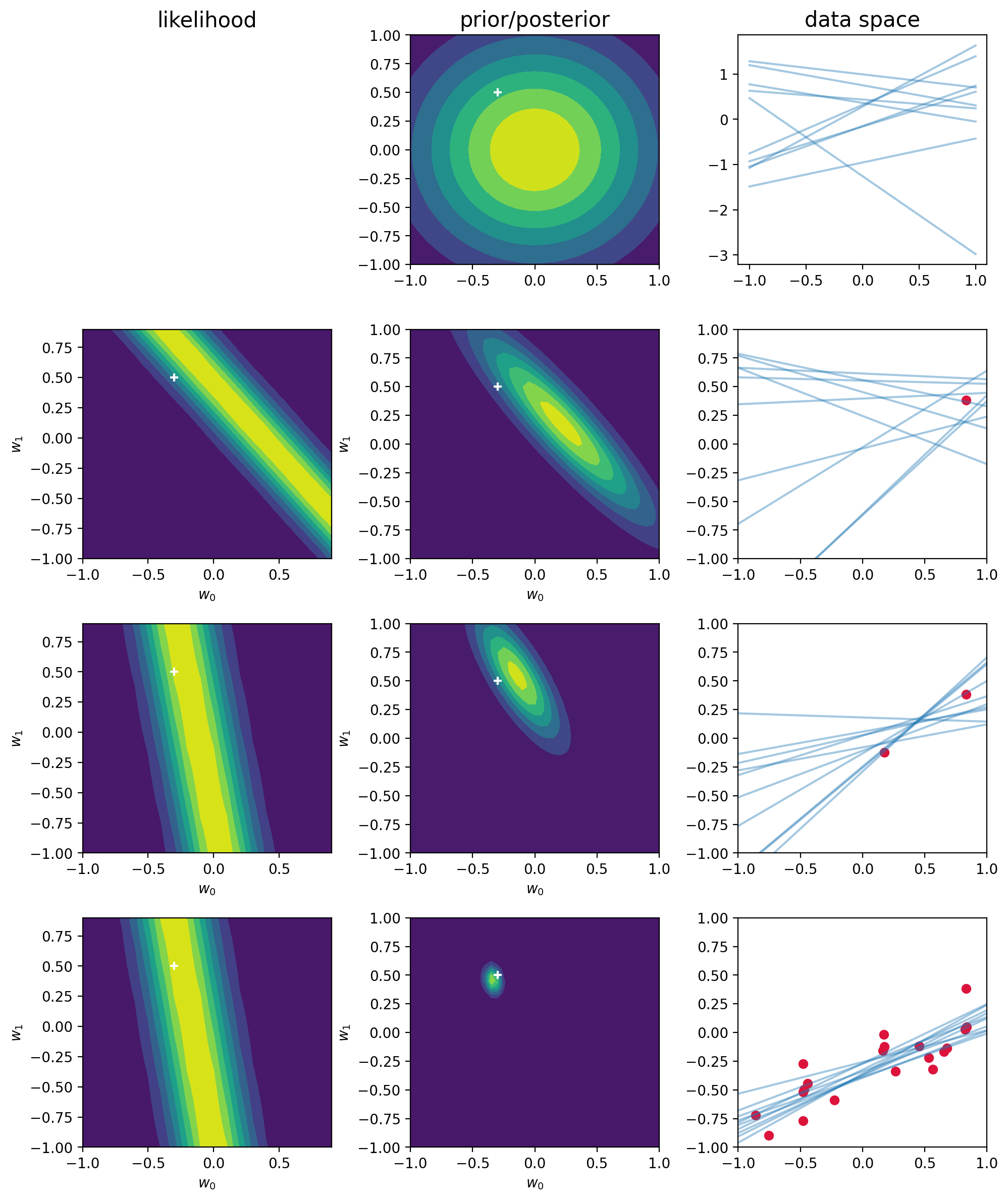

In the limit of an infinite number of datapoints, the posterior distribution would become a delta function centered on the true parameter values, shown by the white cross.

Other forms of prior over parameters can be considered. For example, the generalized Gaussian:

\[ p({\bf w}|\alpha) = \left[\frac{q}{2}\left(\frac{q}{2}\right)^{1/q}\frac{1}{\Gamma(1/q)}\right]^M \exp\left(-\frac{\alpha}{2}\sum_{j=1}^M|w_j|^q\right) \]

Finding the maximum posterior distribution over \({\bf w}\) corresponds to minimization of the regularized error function given by:

\[ \frac{1}{2}\sum_{n=1}^N\left(t_n - {\bf w}^T {\bf\phi}({\bf x}_n)\right)^2 + \frac{\lambda}{2}\sum_{j=1}^{M}|w_j|^q \]

The maximum posterior weight vector \({\bf w}_{\text{MAP}}\) considering a generalized Gaussian will not be (in every case) the mean, since the mean will not coincide with the mode.